An Introduction to Tensorflow
Another topic that falls under machine learning is 'deep learning'. Whereas the machine learning algorithms already covered can be described as linear, or more specialized, deep learning makes use of neural networks that essentially give the algorithm the ability to process the data in a non-linear fashion. Often times neural networks are mentioned to work similarly to the human brain.
The Tensorflow library can be used to code the former kind of machine learning algorithms though it excels at coding neural networks. In particular, Tensorflow will allow you to use the GPU and multiple devices for processing which turns out to be very efficient for deep learning tasks (think parallelism and distributed execution). Tensorflow is a very powerful library and the neural network functionality relies heavily on the understanding of computational graphs. Below are two great resources to follow up on computational graphs:
Theory Behind Computational Graphs
Sample Tensorflow Graph
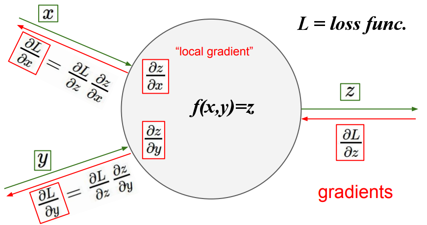
But if you feel like plowing through, here is a very rough description regarding how neural networks function. In a Neural Network all that is happening is the following keeping in mind that, as with other machine learning methods, we want to minimize the loss function:
- start with a set of weights
- loop (such as with gradient descent)
- do the forward pass and at the end compute the loss function
- while doing the forward pass save a various results that will be used in the backward pass
- do the backward pass using the calculations saved during the forward pass
- here you find the analytic gradient (red portions in the computational graph image)
- note that the chain rule of calculus plays a crucial role in this process (red portions in the computational graph image)
- recalculate the weights
- since the gradient is the direction of steepest ascent, chose the weights so that you go in the opposite direction of the gradient
- this will necessarily take you to the location of the minimum
- since the gradient is the direction of steepest ascent, chose the weights so that you go in the opposite direction of the gradient
- reach some halting condition
- do the forward pass and at the end compute the loss function
Tensorflow takes a little getting used to and this is because the code is using a dataflow programming model where first you define the dataflow graph and then you create a session that runs the graph. So it feels like programming in a different paradigm. A more thorough explanation of tensorflow's dataflow programming can be found here. As an example, the code below shows you what a simple multiplication of two values looks like using Tensorflow.
import tensorflow as tf

# Initialize two constants
a = tf.constant(2)
b = tf.constant(6)
# Multiply both constants
result = tf.multiply(a, b)
print(result)

# run session
with tf.Session() as sess:
    print(sess.run(result))
To give an even better idea of how Tensorflow works, below is a comparison of a perceptron algorithm using scikitlearn and the corresponding Tensorflow implementation.
Scikitlearn Implementation of the Perceptron
# Perceptron example using scikitlearn

import tensorflow as tf
import numpy as np
import os
import matplotlib.pyplot as plt

data = np.genfromtxt('input/perceptron_toydata.txt', delimiter='\t')
data
X, y = data[:, :2], data[:, 2]
y = y.astype(np.int)

print('Class label counts:', np.bincount(y))

plt.scatter(X[y==0, 0], X[y==0, 1], label='class 0', marker='o', color='b')
plt.scatter(X[y==1, 0], X[y==1, 1], label='class 1', marker='s', color='orange')
plt.xlabel('feature 1')
plt.ylabel('feature 2')
plt.title('All Perceptron data')
plt.legend()
plt.show()

# Shuffle dataset
# Split dataset into 70% training and 30% test data
# Seed random number generator for reproducibility
# Shuffle the data
shuffle_idx = np.arange(y.shape[0])
shuffle_rng = np.random.RandomState(123)
shuffle_rng.shuffle(shuffle_idx)
X, y = X[shuffle_idx], y[shuffle_idx]
X_train, X_test = X[shuffle_idx[:70]], X[shuffle_idx[70:]]
y_train, y_test = y[shuffle_idx[:70]], y[shuffle_idx[70:]]

# Standardize
mu, sigma = X_train.mean(axis=0), X_train.std(axis=0)
X_train = (X_train - mu) / sigma
X_test = (X_test - mu) / sigma

# Fit on train set and predict on test set
from sklearn.linear_model import Perceptron
p = Perceptron(penalty='l2', alpha = 0.1, fit_intercept = True, max_iter = 2,
               tol = None, shuffle = False)
p.fit(X_train, y_train)
pred_train = p.predict(X_train)
pred_test = p.predict(X_test)

train_errors = np.sum(pred_train != y_train)
print('Number of train errors {0} out of {1}.'.format(train_errors, len(X_train)))
test_errors = np.sum(pred_test != y_test)
print('Number of test errors {0} out of {1}.'.format(test_errors, len(X_test)))

# Graph the results
from mlxtend.plotting import plot_decision_regions
# Train set
plot_decision_regions(X_train, y_train, clf=p)
plt.title('Perceptron train data with decision boundary')
plt.show()

# Test set
plot_decision_regions(X_test, y_test, clf=p)
plt.title('Perceptron test data with decision boundary')
plt.show()


Tensorflow Implementation of the Perceptron
# Perceptron example using tensorflow

g = tf.Graph()
n_features = X_train.shape[1]

with g.as_default() as g:

    # initialize model parameters
    features = tf.placeholder(dtype=tf.float32,
                              shape=[None, n_features], name='features')
    targets = tf.placeholder(dtype=tf.float32,
                             shape=[None, 1], name='targets')
    params = {
        'weights': tf.Variable(tf.zeros(shape=[n_features, 1],
                                        dtype=tf.float32), name='weights'),
        'bias': tf.Variable([[0.]], dtype=tf.float32, name='bias')}

    # forward pass
    linear = tf.matmul(features, params['weights']) + params['bias']
    ones = tf.ones(shape=tf.shape(linear))
    zeros = tf.zeros(shape=tf.shape(linear))
    prediction = tf.where(tf.less(linear, 0.), zeros, ones, name='prediction')

    # weight update
    diff = targets - prediction
    weight_update = tf.assign_add(params['weights'],
                                  tf.reshape(diff * features, (n_features, 1)))
    bias_update = tf.assign_add(params['bias'], diff)

    saver = tf.train.Saver()

with tf.Session(graph=g) as sess:

    sess.run(tf.global_variables_initializer())

    i = 0
    for example, target in zip(X_train, y_train):
        feed_dict = {features: example.reshape(-1, n_features),
                     targets: target.reshape(-1, 1)}
        _, _ = sess.run([weight_update, bias_update], feed_dict=feed_dict)

        i += 1
        if i >= 4:
            break

    modelparams = sess.run(params)
    print('Model parameters:\n', modelparams)

    saver.save(sess, save_path='./perceptron')

    pred = sess.run(prediction, feed_dict={features: X_train})
    errors_train = np.sum(pred.reshape(-1) != y_train)
    pred_test = sess.run(prediction, feed_dict={features: X_test})
    errors_test = np.sum(pred_test.reshape(-1) != y_test)
    print('Number of train errors:', errors_train)
    print('Number of test errors', errors_test)

# Graph the results
plt.scatter(X[y==0, 0], X[y==0, 1], label='class 0', marker='o', color='b')
plt.scatter(X[y==1, 0], X[y==1, 1], label='class 1', marker='s', color='orange')
plt.xlabel('feature 1')
plt.ylabel('feature 2')
plt.title('All Tensorflow data (same as perceptron)')
plt.legend(loc='upper left')
plt.show()

# Graph the results
# calculate the decision boundary
x_min = -2
y_min = (-(modelparams['weights'][0] * x_min) / modelparams['weights'][1] -
         (modelparams['bias'][0] / modelparams['weights'][1]))

x_max = 2
y_max = (-(modelparams['weights'][0] * x_max) / modelparams['weights'][1] -
         (modelparams['bias'][0] / modelparams['weights'][1]))


fig, ax = plt.subplots(2, 1, sharex=False, figsize=(6, 12))
ax[0].plot([x_min, x_max], [y_min, y_max])
ax[1].plot([x_min, x_max], [y_min, y_max])

ax[0].scatter(X_train[y_train == 0, 0], X_train[y_train == 0, 1],
              label='class 0', marker='o', color='b')
ax[0].scatter(X_train[y_train == 1, 0], X_train[y_train == 1, 1],
              label='class 1', marker='s', color='orange')
ax[0].set_title('Perceptron train data with decision boundary')
ax[0].set_xlabel('feature 1')
ax[0].set_ylabel('feature 2')

ax[1].scatter(X_test[y_test == 0, 0], X_test[y_test == 0, 1],
              label='class 0', marker='o', color='b')
ax[1].scatter(X_test[y_test == 1, 0], X_test[y_test == 1, 1],
              label='class 1', marker='s', color='orange')
ax[1].set_title('Perceptron test data with decision boundary')
ax[1].set_xlabel('feature 1')
ax[1].set_ylabel('feature 2')
plt.show()


Admittedly the logistic regression implementation of the perceptron beat out the tensorflow/neural network version. For higher dimensional and more complex scenarios the neural network will beat other methods or be the only practical option.